How to Use Microsoft Excel PivotTables to Analyse Sales, Expenses, Inventory, and Business Records in Nigeria

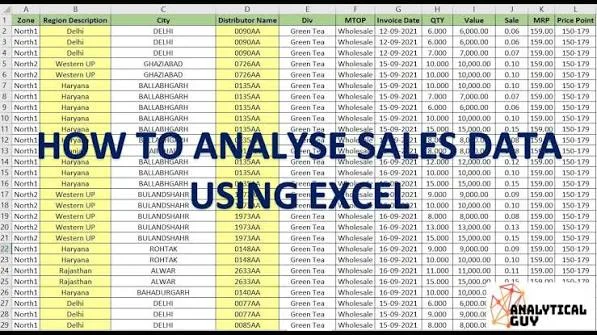
Running a business involves collecting information every day. A retailer records sales, a school tracks payments, a distributor monitors stock, and a freelancer keeps records of income and expenses. As these records grow, finding useful information becomes more difficult. A spreadsheet containing hundreds or thousands of rows may hold everything you need, but manually checking each entry can waste valuable time.

Microsoft Excel PivotTables provide a practical way to organise and analyse large amounts of information without writing complicated formulas. You can use them to calculate total sales, compare monthly revenue, identify popular products, examine customer purchases, track expenses, and understand inventory movements.

For Nigerian business owners, students, accountants, administrative workers, and entrepreneurs, learning PivotTables can make everyday record-keeping more efficient. You do not need to be an advanced Excel user to get started. Once you understand how to structure your data and arrange fields correctly, you can create useful reports in minutes.

This guide explains what PivotTables are, how they work, how to create your first report, and how to apply them to realistic business situations. It also covers common mistakes, troubleshooting, practical examples, and ways to improve your Excel skills.

1. What Is an Excel PivotTable?

A PivotTable is an Excel feature that summarises and analyses information stored in a spreadsheet. Instead of manually adding figures or searching through hundreds of records, you can use a PivotTable to organise information into categories and calculate totals, counts, averages, and other useful measurements.

Imagine that you operate a laptop shop in Lagos. Every day, you record transactions involving different laptop brands, models, customers, payment methods, and sales amounts.

After several months, your spreadsheet may contain hundreds of transactions. You may want to answer questions such as:

• How much revenue did the business generate this month?
• Which laptop brand generated the highest sales?
• How many laptops were sold in each category?
• Which salesperson recorded the highest revenue?
• How much did customers pay through bank transfers?
• Which products generated the lowest sales?
• How did sales change between January and February?

You could calculate these figures manually, but doing so repeatedly becomes inefficient. A PivotTable allows you to rearrange the same information to answer different questions without changing the original transaction records.

The word pivot refers to the ability to change the way information is organised. You can move fields between rows, columns, filters, and values to examine your data from different perspectives.

2. Why Nigerian Businesses Should Learn PivotTables

Many small businesses collect information in Excel but use only basic calculations. They enter transactions, calculate totals, and save the workbook. However, they may not take advantage of the information already stored in their records.

PivotTables help turn those records into reports that support better decisions.

Retail businesses

A retailer can analyse daily transactions to identify popular products, compare sales between branches, and understand which categories contribute most to revenue.

For example, a computer retailer can compare sales of HP, Dell, Lenovo, Apple, and other laptop brands. The results can help the business understand customer demand and plan future purchases.

Schools and educational institutions

A school administrator can use PivotTables to summarise fee payments by class, term, payment status, or academic session. This can help the administration identify outstanding balances and understand payment patterns.

Freelancers and consultants

A freelancer can analyse payments from different clients, compare monthly income, and identify the services generating the most revenue.

Distributors and wholesalers

A distributor can examine product quantities, sales territories, customer orders, and stock movements. This can help identify products that sell quickly and products that remain in storage for too long.

Accountants and administrative workers

Accountants can use PivotTables to summarise transaction records, analyse expense categories, compare departmental spending, and prepare supporting reports.

PivotTables do not replace proper accounting procedures or accounting software. However, they can make spreadsheet-based analysis considerably easier.

3. Prepare Your Data Before Creating a PivotTable

The quality of a PivotTable depends heavily on the quality of the source data. If your spreadsheet contains inconsistent headings, blank rows, merged cells, or incorrectly entered figures, Excel may produce incomplete or confusing results.

Before creating a PivotTable, organise your information into a proper table.

Use one header row

Each column should have a clear heading. For example, a sales spreadsheet might contain these columns:

• Date
• Invoice Number
• Product
• Brand
• Category
• Quantity
• Unit Price
• Salesperson
• Payment Method
• Customer

Every column should describe one type of information. Avoid placing several unrelated details inside a single column.

Do not merge cells in the source data

Merged cells can interfere with sorting, filtering, and PivotTable creation. Keep the source data in a simple rectangular structure, with one heading per column and one transaction per row.

Avoid blank rows and columns inside the data

Do not insert decorative blank rows between transaction records. A completely blank row may cause Excel to interpret the information as separate data ranges.

Use consistent spelling

Suppose you record the same payment method in different ways:

• Bank Transfer
• Bank transfer
• Transfer
• Bank Tfr

Excel may treat these as separate categories. Standardise the descriptions before creating your report.

Enter numbers as numbers

Sales amounts should be stored as numeric values, not text. If you type the naira symbol or explanatory words inconsistently inside cells, Excel may fail to calculate the figures correctly.

You can apply the Nigerian naira currency format to numeric cells without typing the currency symbol into every individual entry.

Use proper dates

Enter dates in a consistent format that Excel recognises. A date stored as text may not group correctly by month or year.

For example, if some entries are recognised as dates and others are stored as text, your PivotTable may display inconsistent results.

4. Create a Sample Sales Dataset in Excel

To understand PivotTables, consider a small Nigerian laptop retailer that records the following transactions.

Date	Product	Brand	Quantity	Unit Price	Payment Method
02/01/2026	EliteBook 840 G6	HP	2	450000	Transfer
03/01/2026	Latitude 5400	Dell	1	380000	Cash
04/01/2026	ThinkPad T480	Lenovo	3	320000	Transfer
06/01/2026	EliteBook 830 G6	HP	1	410000	POS
08/01/2026	Latitude 7400	Dell	2	500000	Transfer
10/01/2026	ThinkPad T490	Lenovo	1	390000	Cash

This is a small sample. A real business may have hundreds or thousands of transactions. The same PivotTable principles apply regardless of the size of the dataset, provided Excel can handle the information and the source data is structured correctly.

For this example, create an additional column called Total Sales. If Quantity is in column D and Unit Price is in column E, enter the following formula in the first data row:

=D2*E2

Copy the formula down the column. Excel will calculate the total value of each transaction.

For the first transaction, two laptops sold at ₦450,000 each produce a total sales value of ₦900,000.

5. Convert Your Data Into an Excel Table

Although you can create a PivotTable from an ordinary cell range, converting the source data into an Excel Table makes the process easier to manage.

To create a table:

1. Click any cell inside your sales data.
2. Press Ctrl + T.
3. Check that Excel has selected the complete data range.
4. Ensure the My table has headers option is selected.
5. Click OK.

Excel will format the data as a table. You can also change the table name through the Table Design tab.

Use a meaningful name such as SalesData. Avoid spaces in table names because Excel table names have naming restrictions.

One major advantage of using an Excel Table is that new rows added directly below the table can become part of its data range automatically. This makes it easier to refresh reports as your business records grow.

6. How to Create Your First PivotTable

Once your data is ready, you can create your first PivotTable.

Step 1: Select your data

Click any cell inside the Excel Table you created. You do not need to select every row manually if your information is already formatted as a table.

Step 2: Open the Insert tab

Click Insert on the Excel ribbon. Find the PivotTable option and select it.

Step 3: Choose the data source

Excel should automatically identify your table as the source. Confirm that the correct table name or data range appears in the dialog box.

Step 4: Choose where to place the PivotTable

You can place the PivotTable on a new worksheet or an existing worksheet. For beginners, a new worksheet is usually easier because it keeps the original transaction records separate from the report.

Step 5: Click OK

Excel will create an empty PivotTable and display the PivotTable Fields panel. This panel contains the headings from your original data.

You can now drag the fields into different areas to build your report.

7. Understand the Four Main PivotTable Areas

The PivotTable Fields panel contains four important areas: Filters, Columns, Rows, and Values. Understanding their functions makes it easier to create different reports.

Rows

The Rows area determines which categories appear vertically in your report.

For example, dragging Brand into Rows displays HP, Dell, Lenovo, and other brands as separate entries.

Columns

The Columns area places categories horizontally across the report.

If you place Payment Method in Columns, Excel can display Transfer, Cash, and POS as separate column headings.

Values

The Values area contains the calculations. You can use it to display total sales, total quantities, average prices, or transaction counts.

For example, dragging Total Sales into Values may automatically calculate the sum of all sales amounts.

Filters

The Filters area allows you to filter the entire report using a selected field.

You could place Date in Filters to examine transactions from a particular period, or place Salesperson there to focus on one employee’s performance.

8. Example One: Calculate Total Sales by Laptop Brand

Suppose you want to know which laptop brand generates the highest sales revenue.

Follow these steps:

1. Drag Brand into the Rows area.
2. Drag Total Sales into the Values area.
3. Confirm that Excel displays Sum of Total Sales.

Your PivotTable will now group transactions by brand and calculate the total sales value for each brand.

This report can help a retailer compare product categories and understand where revenue comes from.

For example, if HP generates ₦12 million in sales, Dell generates ₦9 million, and Lenovo generates ₦5 million, you can immediately see how the brands compare.

These figures are illustrative, not actual market or P-Sero sales figures.

Change the calculation if necessary

Excel sometimes chooses Count instead of Sum, particularly when the source column contains numbers stored as text or a mixture of numeric and non-numeric entries.

To change the calculation:

1. Click the drop-down arrow beside the field in the Values area.
2. Select Value Field Settings.
3. Choose Sum.
4. Click OK.

If Sum is unavailable or the result remains incorrect, inspect the source column for text values, blank entries, or inconsistent data.

9. Example Two: Calculate Monthly Sales

Monthly sales reports are useful for identifying changes in business performance. Instead of calculating each month manually, you can group transaction dates inside a PivotTable.

To create a monthly sales report:

1. Drag Date into the Rows area.
2. Drag Total Sales into the Values area.
3. Right-click one of the date entries in the PivotTable.
4. Select Group.
5. Choose Months and Years where available.
6. Click OK.

Excel will organise your transactions by month and year.

Including the year is important when your dataset contains more than one year. Otherwise, January 2025 and January 2026 could appear together in a report that groups only by month.

You can now compare January, February, March, and other months to identify periods with higher or lower revenue.

10. Example Three: Find the Most Popular Products

A business may generate high revenue from a few expensive products while selling larger quantities of cheaper products. Revenue alone does not tell you which products are most popular by volume.

To find the most frequently sold products:

1. Drag Product into Rows.
2. Drag Quantity into Values.
3. Confirm that the calculation is Sum of Quantity.
4. Sort the results from largest to smallest.

The report will show the total quantity sold for each product.

This information can help a retailer identify products that customers buy frequently. It can also support stock planning and purchasing decisions.

However, remember that high sales volume does not automatically mean high profitability. A product that sells frequently may have a small profit margin.

11. Example Four: Analyse Sales by Payment Method

Nigerian businesses often receive payments through bank transfers, POS transactions, cash, and other payment channels. Understanding how customers pay can help with reconciliation and transaction monitoring.

To create a payment-method report:

1. Drag Payment Method into Rows.
2. Drag Total Sales into Values.
3. Check that the calculation is Sum.

You can also drag Quantity or Invoice Number into Values to examine the number of units sold or transactions recorded through each method.

If you want to count transactions, use a field that has a value for every transaction, such as Invoice Number, and select Count under Value Field Settings.

This report can help you compare the volume and value of payments received through different channels. It does not replace checking your bank statements, POS settlement reports, or cash records.

12. Example Five: Compare Salespeople

If your business has several sales representatives, you can use PivotTables to compare their recorded sales.

Place Salesperson in Rows and Total Sales in Values. Excel will calculate the total sales attributed to each employee.

You can also add Product to Columns to compare which categories each salesperson sells most frequently.

For example, one salesperson may generate more revenue from premium laptops, while another may sell a larger quantity of entry-level devices.

Use the results as one part of performance evaluation. Consider factors such as returns, discounts, customer satisfaction, and profit margins before drawing conclusions about employee performance.

13. How to Filter a PivotTable

As your reports become more detailed, filters help you focus on the information that matters.

For example, you may want to analyse sales from January only, or examine transactions involving HP laptops.

Use a report filter

Drag a field such as Brand or Payment Method into the Filters area. A filter will appear above the PivotTable. Open its drop-down menu and select the category you want to examine.

Use row and column filters

Fields placed in Rows and Columns usually include drop-down filtering options. These allow you to show or hide particular categories without changing the source data.

Use search inside a filter

If the field contains many products or customers, use the search box in the filter menu to locate a specific entry.

Filtering does not delete the original records. It changes which records appear in the report.

14. Use Slicers to Make Reports Easier to Navigate

A slicer is a visual filtering tool that allows you to filter a PivotTable by clicking buttons.

Instead of opening a drop-down menu, you can click a category such as HP, Dell, Transfer, or Cash.

How to insert a slicer

1. Click anywhere inside your PivotTable.
2. Open the PivotTable Analyze tab.
3. Select Insert Slicer.
4. Choose the fields you want to use as filters.
5. Click OK.

Excel will create slicer panels that you can position beside your report.

Slicers are particularly useful when preparing reports for business owners or managers who may not be comfortable navigating Excel’s field filters.

Clear a slicer selection

Use the clear-filter icon on the slicer to return to the full dataset. This is useful when you have filtered several categories and want to see all records again.

15. Group Data by Month, Quarter, and Year

Grouping dates helps you analyse performance over different periods.

A business may want to compare monthly revenue, examine quarterly performance, or review annual results.

When your source contains valid Excel dates, you can right-click a date in the PivotTable, select Group, and choose suitable time periods.

Depending on your version of Excel and the source data, you may be able to group by:

• Days
• Months
• Quarters
• Years

You can select multiple grouping levels when appropriate. For example, grouping by Months and Years allows you to see January, February, and March separately for each year.

If Excel refuses to group the dates, check whether the source column contains blank cells, text values, or invalid dates.

16. Use PivotTables to Analyse Business Expenses

PivotTables are not limited to sales. You can also use them to analyse business expenses.

Suppose you record expenses using the following headings:

• Date
• Expense Category
• Description
• Department
• Payment Method
• Amount

Expense categories might include rent, electricity, internet, transport, salaries, repairs, advertising, packaging, and office supplies.

To summarise expenses by category:

1. Create a PivotTable from the expense records.
2. Drag Expense Category into Rows.
3. Drag Amount into Values.
4. Confirm that Excel uses Sum of Amount.
5. Sort the results from highest to lowest.

The report will show which categories account for the largest recorded expenses.

You can also place Department in Columns to compare spending between departments or use Date to examine monthly changes.

This can help business owners identify spending patterns and investigate unusual increases.

17. Use PivotTables to Track Inventory

Inventory management is another area where PivotTables can be useful. A retailer needs to know what was purchased, what was sold, and what remains in stock.

A simple inventory movement spreadsheet could contain:

• Date
• Product
• Product Category
• Movement Type
• Quantity
• Supplier
• Reference Number

Movement Type could identify whether a record represents stock received, stock sold, returned stock, or an adjustment.

You can create a PivotTable that places Product in Rows, Movement Type in Columns, and Quantity in Values.

This report can show quantities associated with each type of movement. However, it does not automatically calculate accurate closing stock unless your data structure and calculations account for opening balances, incoming stock, outgoing stock, returns, and adjustments correctly.

For a simple stock calculation, you can use:

Closing Stock = Opening Stock + Stock Received - Stock Sold

Returns and authorised adjustments should be handled separately according to how your business records inventory movements.

For a laptop retailer, this approach can help monitor quantities of different models and identify products that need restocking.

18. Calculate Average Sales, Maximum Sales, and Minimum Sales

PivotTables can do more than calculate totals. You can change the summary calculation to examine averages, minimum values, maximum values, and counts.

To change a calculation:

1. Click the field inside the Values area.
2. Open Value Field Settings.
3. Select the required calculation.
4. Click OK.

Common calculations include:

• Sum: adds all numeric values.
• Count: counts records containing values.
• Average: calculates the average of numeric entries.
• Max: displays the largest value.
• Min: displays the smallest value.

For example, you can calculate the average transaction value for each salesperson or identify the highest recorded sale for each product category.

Be careful when interpreting averages. An average selling price may be distorted by unusual transactions, discounts, or bulk orders.

19. Show Values as Percentages

Sometimes a business owner wants to know what percentage of total sales comes from each category rather than simply viewing the naira amounts.

PivotTables can display values as percentages of a grand total, row total, or column total.

How to show percentage of grand total

1. Click a value inside the PivotTable.
2. Open Value Field Settings.
3. Select the Show Values As tab.
4. Choose % of Grand Total.
5. Click OK.

Excel will display each category’s contribution to the overall total.

For example, if HP accounts for 50% of recorded sales, Dell accounts for 30%, and Lenovo accounts for 20%, the report makes the distribution easier to understand.

These percentages describe the dataset being analysed. They should not be presented as market share unless the data genuinely represents the wider market.

20. Sort PivotTable Results to Find Important Information

Sorting helps you identify the highest and lowest values in a report.

Suppose you have a PivotTable showing total revenue by product. To find the products generating the highest sales:

1. Click a value in the Sum of Total Sales column.
2. Right-click the value.
3. Select Sort.
4. Choose Largest to Smallest.

You can reverse the order to find the lowest recorded sales.

This is useful when reviewing product performance, employee sales, customer purchases, or expense categories.

21. Create a PivotChart From Your Report

A PivotChart turns PivotTable information into a visual chart. It can help people understand patterns without studying a large table of figures.

To create one:

1. Click inside the PivotTable.
2. Open the Insert tab.
3. Select PivotChart, where available.
4. Choose a suitable chart type.
5. Click OK.

Common chart choices include:

• Column charts for comparing sales between product categories.
• Bar charts for ranking products or employees.
• Line charts for examining monthly sales trends.
• Pie or doughnut charts for showing a small number of category proportions.

Avoid using a complicated chart when a simple table communicates the information more clearly. For example, a report with 40 product categories may be easier to understand as a sorted table than as a pie chart with dozens of slices.

22. Refresh a PivotTable When New Data Is Added

A PivotTable does not always update automatically when you change the original records. If you add new transactions, refresh the report to include the latest information.

Refresh one PivotTable

1. Click inside the PivotTable.
2. Right-click.
3. Select Refresh.

You can also use the Refresh option under the PivotTable Analyze tab.

Refresh all reports

If your workbook contains several PivotTables, use Data and select Refresh All. This updates the workbook’s supported data connections and PivotTables.

Why Excel Tables are helpful

If your source data is formatted as an Excel Table, newly added records can become part of the table automatically. After adding the records, refresh the PivotTable to include them.

If your PivotTable uses a fixed cell range rather than an Excel Table, you may need to change the source data range when new rows are added.

23. Common PivotTable Problems and How to Fix Them

Excel displays Count instead of Sum

This often happens when a supposed numeric column contains text, blank entries, or inconsistent values. Check the source data and convert valid numbers stored as text into real numeric values. Then refresh the PivotTable and change the summary calculation to Sum.

New records do not appear

Refresh the PivotTable. If the source uses a fixed range, check whether the new records fall outside that range. Consider converting the source data into an Excel Table.

Dates cannot be grouped

Check the source date column for blank cells, text-formatted dates, and invalid entries. Correct the records and refresh the PivotTable.

Duplicate categories appear

Check for inconsistent spelling, extra spaces, and different descriptions of the same item. For example, HP EliteBook and HP Elitebook may be treated as separate labels.

Standardise the source data before refreshing the report.

The PivotTable displays blank categories

This usually indicates missing information in the corresponding source column. Review the original records and fill in the missing values where appropriate.

The report is too wide

You may have placed too many fields in the Columns area. Move some fields to Filters or Rows, or remove fields that are not essential to the report.

Excel cannot create the PivotTable

Check that the source data has a valid header row, contains no merged cells, and uses a consistent rectangular structure. Also confirm that every column has a heading.

24. Protect Your Business Records When Using PivotTables

Business spreadsheets can contain customer names, phone numbers, financial records, supplier details, and other sensitive information. A PivotTable does not automatically protect this information.

Take reasonable steps to protect your workbook.

Keep an original copy

Maintain a backup of the original transaction records before making major changes. A PivotTable summarises information, but it should not replace your source records.

Restrict access to sensitive workbooks

Use appropriate file permissions and password protection where necessary. Do not share customer or financial information publicly.

Use secure storage

Store important workbooks in a reliable location and maintain backups. Consider a suitable cloud storage service or an external backup drive, depending on your business requirements.

Do not treat a PivotTable as proof that records are correct

A PivotTable can summarise incorrect data accurately. If an employee enters the wrong amount, records a transaction twice, or assigns a sale to the wrong product, the report may still calculate a total without warning you that the source information is inaccurate.

Always review the underlying records and reconcile important financial reports against reliable transaction evidence.

25. PivotTables in Excel for Microsoft 365, Excel 2024, and Older Versions

PivotTables have been available in Excel for many years. Most modern desktop versions of Excel support the main PivotTable features discussed in this guide.

However, the location of certain commands, available chart options, and advanced analysis features can vary between Excel versions and platforms.

Microsoft 365 users may receive feature updates over time, while perpetual versions such as Excel 2024 follow a different update model.

Excel for the web also supports PivotTable operations, although some advanced functions may be limited compared with the desktop application.

If you use Excel regularly for business reporting, confirm that your version supports the functions you need. You can find information through Microsoft Excel Support.

26. Practical Exercises to Improve Your PivotTable Skills

The best way to learn PivotTables is to practise with realistic data. Create a sample workbook containing at least 50 transactions. Include dates, products, quantities, prices, customers, payment methods, and salespeople.

Then complete the following exercises.

Exercise 1: Calculate total revenue

Create a PivotTable that shows total sales by product. Sort the results from highest to lowest.

Exercise 2: Compare monthly performance

Group your transaction dates by month and year. Display total revenue for each period.

Exercise 3: Analyse payment methods

Calculate total sales and transaction counts for bank transfers, cash, and POS payments.

Exercise 4: Identify popular products

Summarise total quantities sold by product. Identify the five products with the highest sales volume.

Exercise 5: Review expenses

Create a separate expense dataset and calculate spending by category and month.

Exercise 6: Build a visual report

Create a PivotChart from your monthly sales report. Add a slicer that allows users to filter the report by product brand.

These exercises will help you understand how different fields work together. They also provide practical experience that can be useful in administrative, accounting, retail, and data-entry roles.

27. How PivotTable Skills Can Improve Your Career Opportunities

Excel remains a widely used tool in Nigerian workplaces. Employers in retail, banking, education, logistics, administration, accounting, and operations may expect workers to understand spreadsheet-based reporting.

Knowing how to create a PivotTable can help you move beyond basic data entry.

For example, an administrative assistant who can summarise attendance records, an accountant who can analyse expenses, or a sales officer who can compare monthly revenue may contribute more useful information to their organisation.

PivotTables are also a foundation for more advanced data analysis. Once you understand them, you can progress to formulas, charts, Power Query, Power Pivot, and Microsoft Power BI.

However, do not assume that knowing PivotTables alone makes someone a professional data analyst. Accurate data preparation, business understanding, interpretation, communication, and other analytical skills remain important.

28. Frequently Asked Questions About Excel PivotTables

Do I need advanced Excel knowledge to use PivotTables?

No. Beginners can create useful PivotTables by learning how to prepare data and drag fields into Rows, Columns, Values, and Filters. More advanced reports require additional practice.

Can I create a PivotTable without formulas?

Yes. PivotTables can calculate sums, counts, averages, maximum values, and minimum values without requiring you to write separate formulas for every category.

Can a PivotTable calculate profit?

Yes, if your source data contains the information needed to calculate profit. For example, you can create a Profit column using revenue minus cost and then summarise the result in a PivotTable. Make sure the cost data includes the expenses relevant to the profit figure you intend to report.

Can I use PivotTables for thousands of records?

Yes. PivotTables are designed to summarise substantial datasets. Performance depends on the amount of data, workbook structure, computer specifications, and Excel version.

Can I use a PivotTable to find duplicate transactions?

You can use a PivotTable to count repeated invoice numbers or transaction references, which may help identify possible duplicates. However, you should investigate the original records before deleting anything. Two legitimate transactions may share other similar details.

Can I edit information directly inside a PivotTable?

Normally, you edit the original source data rather than the summarised PivotTable cells. After making changes to the source records, refresh the report.

Can I create several PivotTables from one dataset?

Yes. You can create different reports from the same source data. One PivotTable may summarise sales by brand, another by month, and another by payment method.

Can I use PivotTables for school fee records?

Yes. You can summarise recorded payments by class, term, student, or payment status. Protect student information and verify the source records before using the report for financial decisions.

Are PivotTables available in Excel for the web?

Excel for the web supports PivotTables, although certain advanced features may require the desktop application. Check Microsoft’s current documentation for platform-specific limitations.

Can I send a PivotTable report to someone who does not use Excel?

Yes. You can export or save a report as a PDF, or copy its results into another document. Before sharing, check that the report contains only information the recipient is authorised to see.

Conclusion: Turn Ordinary Excel Records Into Useful Business Reports

Microsoft Excel PivotTables make it easier to understand information stored in spreadsheets. Instead of manually calculating every category, you can summarise sales, expenses, inventory, customer transactions, and business performance using a flexible reporting tool.

For Nigerian retailers, accountants, school administrators, freelancers, and business owners, this can save time and improve the way everyday records support decisions.

Start with a clean dataset, convert it into an Excel Table, and create a simple report using Rows and Values. Once you understand the basics, practise filtering, grouping dates, sorting results, using slicers, and creating PivotCharts.

At P-Sero Laptop, we recognise that a reliable laptop is an important tool for learning Excel, managing business records, and developing professional skills. Whether you are a student, entrepreneur, accountant, or office worker, choosing a suitable laptop can make your daily computing tasks easier.

Explore available laptops at P-Sero Laptop. If you need assistance choosing a laptop for Microsoft Excel, accounting applications, business management, or other professional tasks, contact our team through WhatsApp on +234 907 193 4883.

Useful Official Resources

• Microsoft Excel Support – Official help and guidance for Excel features.
• Microsoft: Create a PivotTable to Analyse Worksheet Data – Step-by-step guidance for creating PivotTables.
• Microsoft: Refresh PivotTable Data – Guidance on updating PivotTable reports.
• Microsoft: Use Slicers to Filter Data – Learn how to add visual filters to reports.